The Mala Knot Lab
Findings
One fact about the number 108, and what follows from it, from a knot to a one-particle quantum system. Read it plain, or switch to Technical for the formulas, the numbers and the file that produced each one. The lab lets you play with all of it, and the replication page lets you check it. None of it is about consciousness, the brain or any theory on this site; section 11 says exactly what it does and does not claim.
In One Paragraph
108 is the usual number of beads on a mala. Leaving aside 1 × 10⁸, it splits into two numbers with nothing in common in only one way, 4 × 27, so 108 beads can be strung on a single knotted loop in exactly one way. We built a model of that knot, and inside it are 27 little four-bead squares. Treat one square as a quantum system and a particle placed on one corner moves to the opposite corner with certainty; physicists call that perfect state transfer, and the four-bead square is the only ring that can do it. So among the common mala counts, 108 is the only one whose split produces rings with that property. Whether the squares survive on a real wound chain depends on the tube being thin; on a fat one they do not. The mathematics of the square is old; placing it on the thread so its corners become neighbours is, as far as we could find, ours; and none of it says anything about consciousness.
1. The One Fact
108 splits cleanly in exactly one way
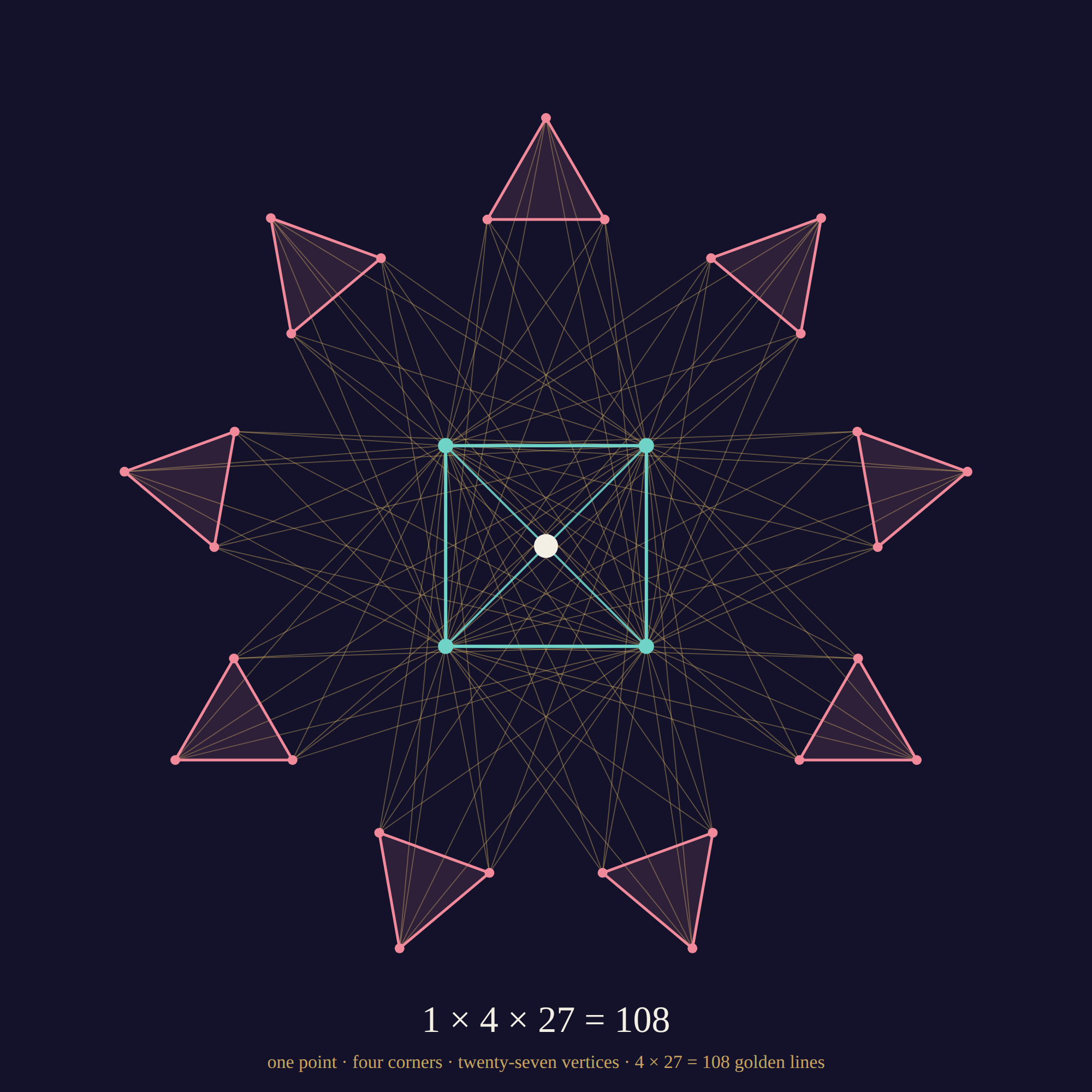
108 has twelve divisors, which pair up into six ways of writing it as one number times another. Leaving aside 1 × 10⁸, only one pair shares nothing: 4 and 27. Every other pair, like 12 and 9 or 6 and 18, has a factor in common. That single clean split is the whole reason the rest of this page exists.
Technical
108 = 2² × 3³. Two factors with no common factor must take all of the 2s or none of them, and all of the 3s or none of them. So the coprime splits are exactly 1 × 10⁸ and 4 × 27, and with both factors greater than 1, 4 × 27 is the only one. (In the language of number theory: 108 has four unitary divisors, 1, 4, 27 and 108.) The same count for the other common mala sizes is in Experiment 2, test 4: 27 = 3³ has no such split, 54 has one (2 × 27), and 1008 = 2⁴ × 3² × 7 has three.
2. The Knot
One thread, 4 laps, 27 turns, 108 beads
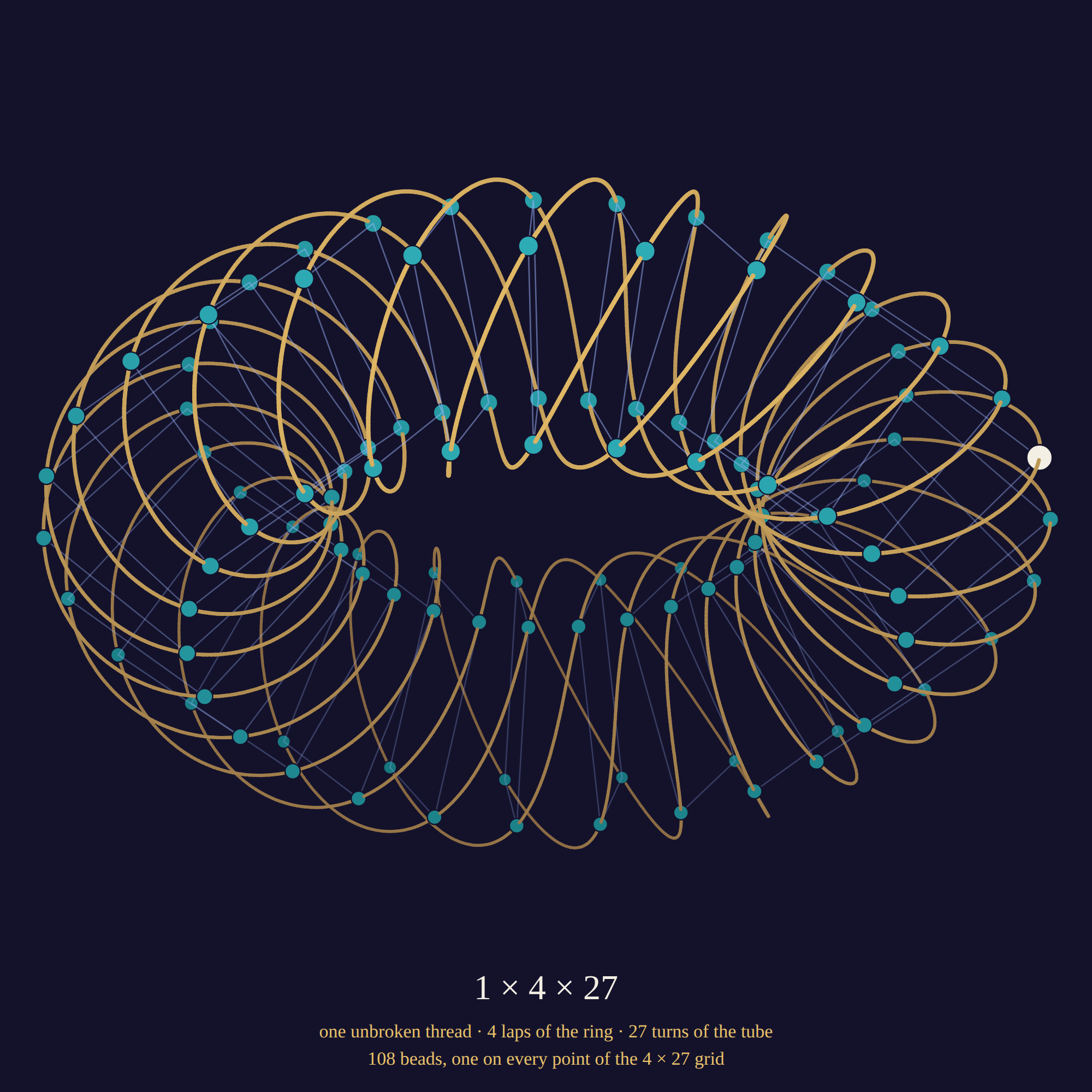
Wind one thread around a doughnut 4 times the long way and 27 times the short way, and it comes back to its start as a single loop. Space 108 beads along it and each bead lands on its own crossing of the 4 × 27 grid. Try 12 and 9, or 6 and 18, and you get several separate loops instead of one.
Technical
The thread is the torus knot T(4, 27). With s running from 0 to 1, the lab places it at angle u = 2π·4s around the ring and v = 2π·27s around the tube. A (p, q) torus curve closes into gcd(p, q) separate components, and gcd(4, 27) = 1, so it is one thread. For (12, 9) the same curve falls into 3 loops; for (6, 18), into 6.
Bead k (k = 0, …, 107) sits at s = k/108, so u = 2πk/27 and v = 2πk/4: station k mod 27 around the ring, corner k mod 4 around the tube. Because 4 and 27 are coprime, the map k ↦ (k mod 27, k mod 4) is one to one (the Chinese remainder theorem), so the 108 beads fill the 27 × 4 grid exactly once each.
Two standard invariants: the crossing number of T(p, q) is min(p(q − 1), q(p − 1)) (Murasugi, 1991), here min(104, 81) = 81; the genus is (p − 1)(q − 1)/2 = 39.
An aside. Torus knots have a known correspondence with the Virasoro minimal models (Hikami and Kirillov, 2003), and the minimal model with labels (4, 27) has 39 primary fields, the same expression as the genus, and central charge −511/18. It is not unitary, and no physical system is known to realise it: the number picked the model, not the other way round. Table: minimal-model-M4-27.md.
3. Shapes
Shapes that survive bending
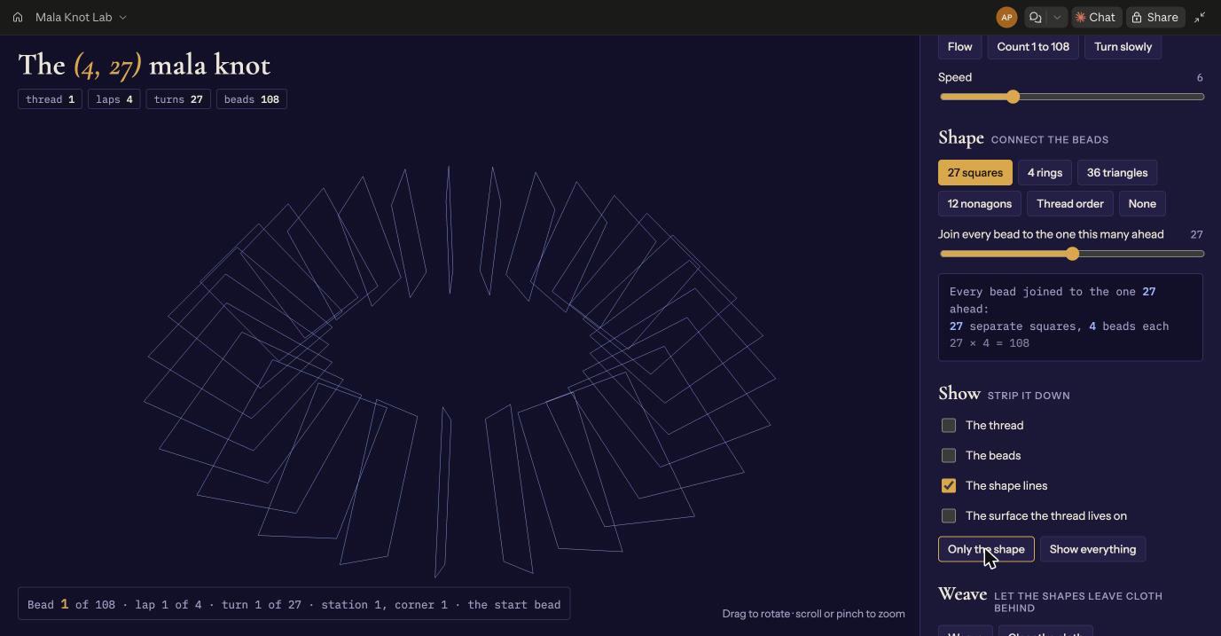
Join every 27th bead and you get 27 squares; every 4th, 4 rings; every 36th, 36 triangles. Bend the thread however you like: the shapes stretch but never break, because each bead keeps its place in the grid.
Technical
Joining each bead k to k + n (mod 108) splits the 108 beads into the cosets of the subgroup generated by n. That subgroup has 108 / gcd(n, 108) elements, so the lines form gcd(n, 108) closed polygons of 108 / gcd(n, 108) beads each: 27 squares for n = 27, 4 rings of 27 for n = 4, 36 triangles for n = 36, 12 nonagons for n = 12, and one loop through all 108 for any n coprime to 108.
The bead address (lap ⌊k/27⌋, turn ⌊k/4⌋, station k mod 27, corner k mod 4) depends on k alone. The thread controls (ring and tube size, petals, rise and fall, cross-section, twist) change only where the torus sits in space, never the order of beads along the thread. So every polygon is defined before any geometry is chosen, and no bending can break it. For n = 27, beads k and k + 27 share a station and differ by one corner, so each square is the tube’s cross-section at one station. For n = 4, the corner stays fixed and the station steps by 4, which visits all 27 stations because 4 and 27 are coprime.
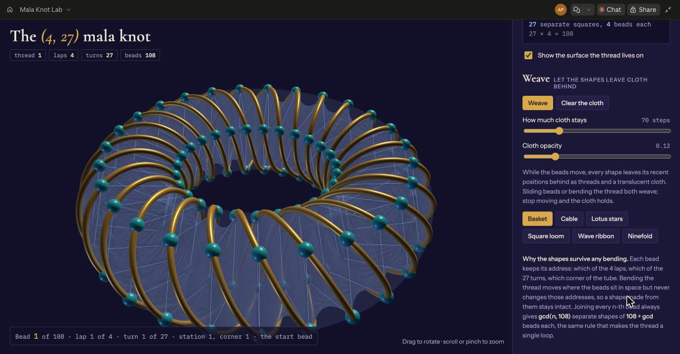
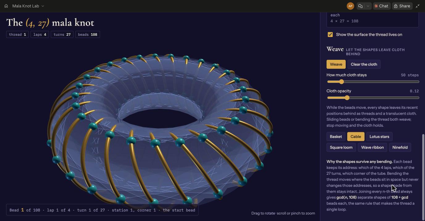
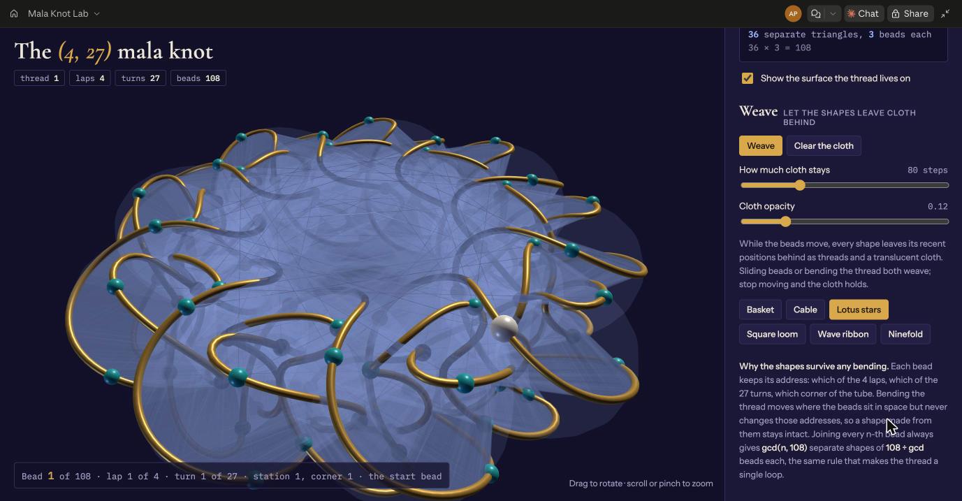
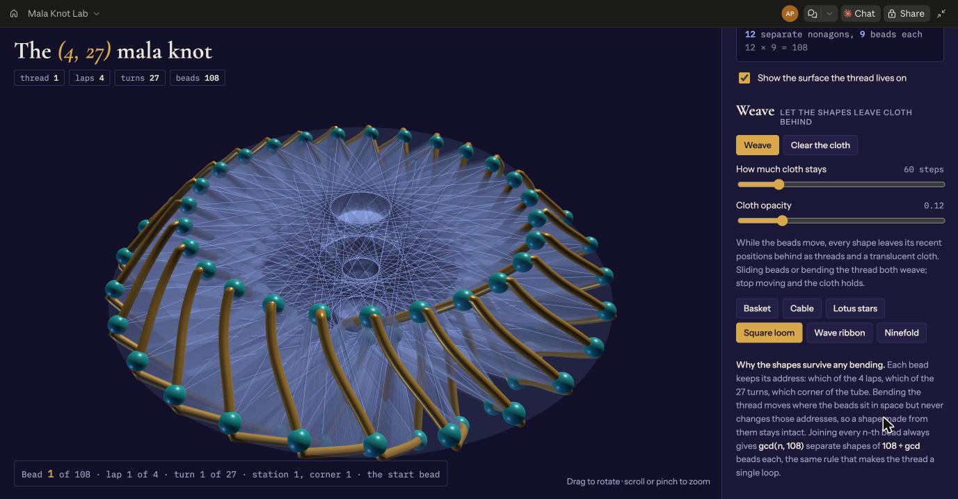
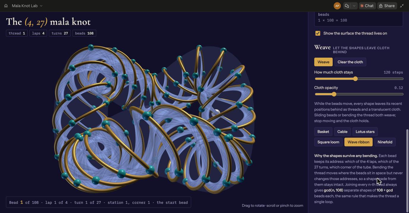
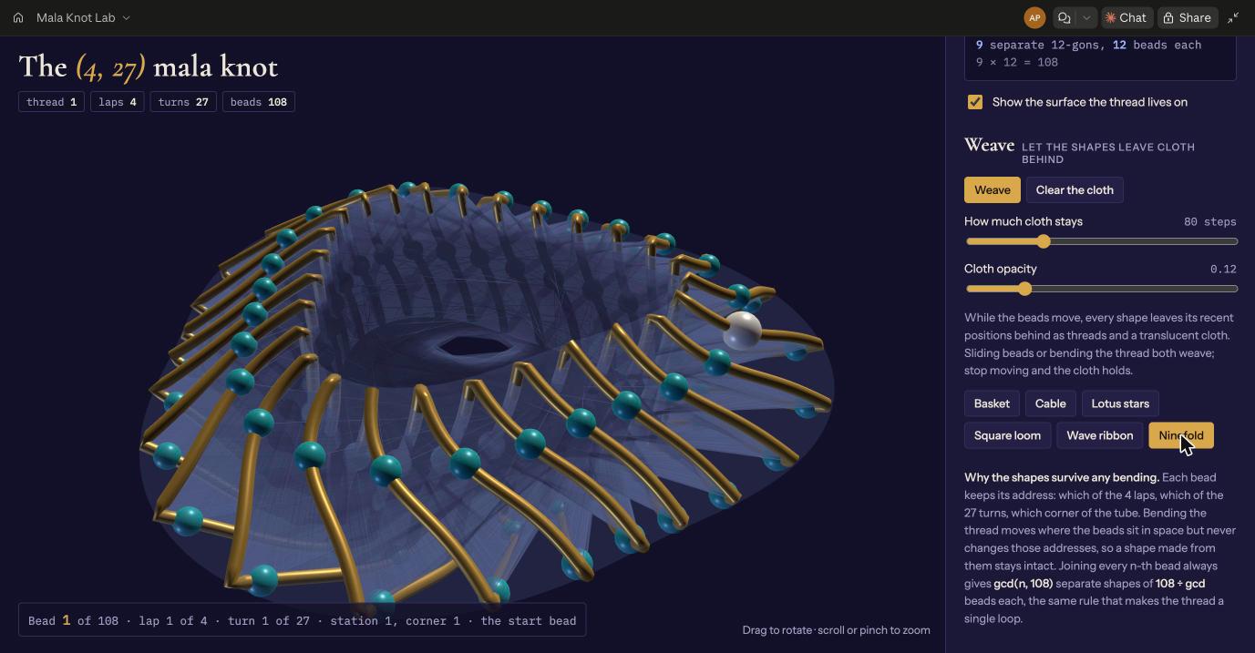
The six weaves in the lab: each is a thread preset, a join step and a flow of beads, with every shape leaving its recent positions behind as cloth. They are drawings of the same arithmetic, not additional results.
4. Found Before
Where the rule was found before
People in Angola, Tamil Nadu and on sailing ships all discovered the same rule by hand: a pattern whose two counts share no factor can be drawn as one unbroken line. We found no one who had drawn it as a mala.
Technical
- Chokwe sona, Angola. Gerdes (1988, 1990) showed that the “plaited-mat” sand drawings on a grid of rows and columns are drawn as a single line only when the two numbers are relatively prime.
- Kolam, Tamil Nadu. Siromoney and Chandrasekaran (1986) showed that a family of kolam with m arms of n dots each is drawn with hcf(m, n) unending lines. Siromoney, Siromoney and Krithivasan (1974) first described kolam with array grammars; Ishimoto (2007) counts single-line kolam with knot theory.
- Turk’s head knots. Ashley (1944, p. 233) gives the “Law of the Common Divisor”: a Turk’s head cannot be tied with one line when its leads and bights share a common divisor. Di Prisa and Şavk (2024) survey Turk’s head knots as mathematical knots and links, with an appendix on torus knots.
- Woven fabric. Grünbaum and Shephard (1980, 1988) set out the geometry of woven fabrics; Yoshida (2026) treats weaves as links in a thickened torus; Dresselhaus and colleagues (2026) review textiles from yarn to topology.
- Beaded torus knots. Chuang and Jin (Bridges, 2014) build beaded models of torus knots T(p, q) with p and q coprime.
Each is cited for what it published, and nothing more; full references are in section 13. The mala reading is ours: as far as we could find, nobody had put a torus knot and a mala together.
5. The Quantum Mode
The quantum mode, and what it is
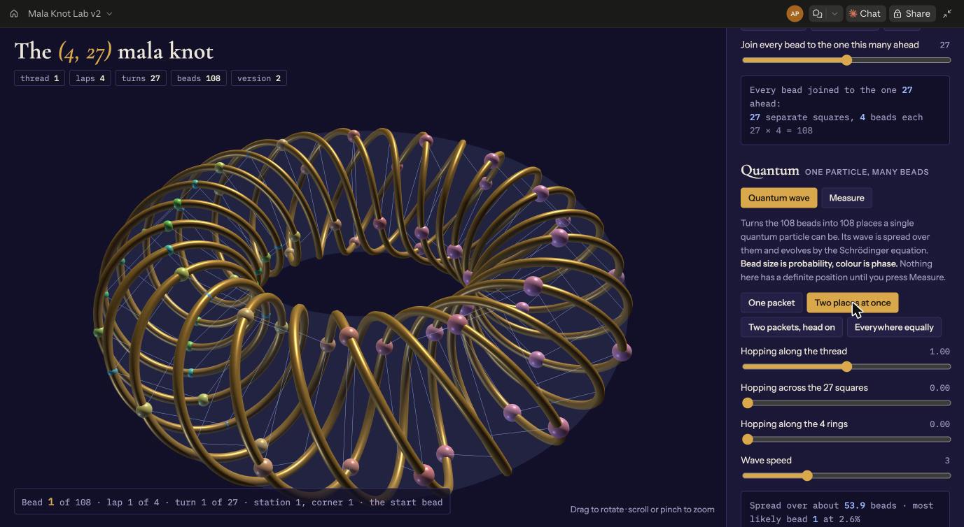
The beads stop being objects and become places where one particle could be. Its wave spreads over them; size shows the odds, colour shows the wave’s phase. Press Measure and it lands on one bead.
It is one particle on a network of 108 places. It is not a model of a mala, a meditator or a mind.
Technical
The state is a vector ψ ∈ ℂ¹⁰⁸, and |ψₖ|² is the probability of finding the particle at bead k + 1. The Hamiltonian is built from three hopping rules, each a step s with a strength tₛ ≥ 0: thread (s = 1), squares (s = 27) and rings (s = 4), all mod 108:
H = −Σₛ tₛ Σₖ ( |k⟩⟨k+s| + |k+s⟩⟨k| ), i dψ/dt = Hψ (ħ = 1).
With all three rules on, the bead network is the Cayley graph of the cyclic group ℤ₁₀₈ with generator set {±1, ±4, ±27}. Each hopping rule alone is a circulant graph, and so H is real, symmetric and circulant: its eigenvectors are the Fourier modes e^(2πink/108), and its eigenvalues are
E(n) = −2[t₁·cos(2πn/108) + t₂₇·cos(πn/2) + t₄·cos(2πn/27)], n = 0, …, 107,
with t₁, t₂₇, t₄ the three hopping strengths. The 4 × 27 structure shows as the periods 4 and 27 of the second and third terms. The thread’s shape appears nowhere in it. On the page, the lab integrates with fourth-order Runge-Kutta, six substeps per frame, renormalising after each step. The tests use exact diagonalisation (numpy.linalg.eigh). Measure draws a bead with probability |ψₖ|² and collapses the state onto it.
6. Experiment 1
Two places at once
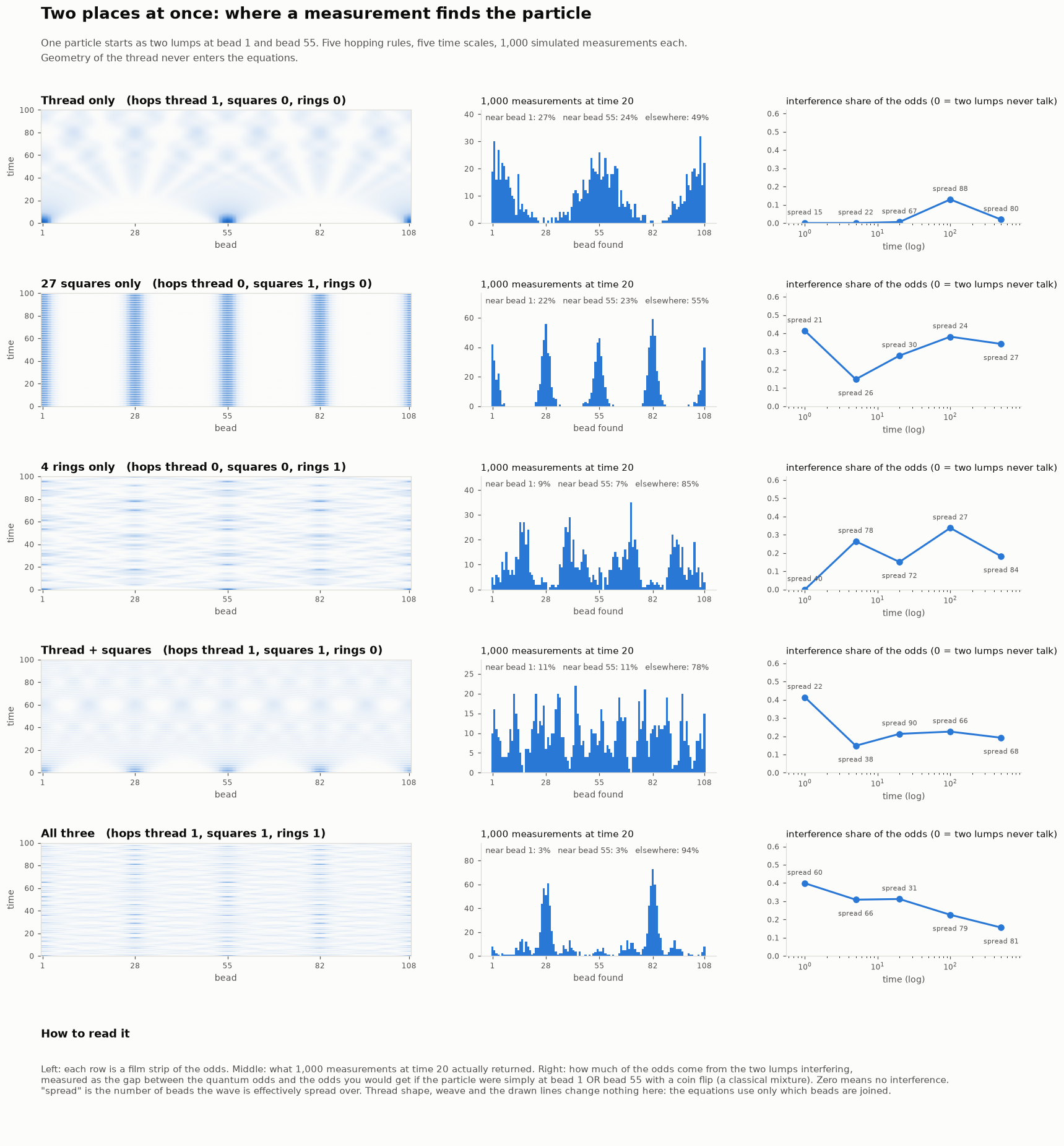
The shape of the thread changes nothing, because the equations never see it. What changes the odds is which beads are allowed to talk to which. With square hopping, the particle keeps turning up at beads 28 and 82, corners where it never started.
Technical
Setup. One particle starts as two equal Gaussian packets, three beads wide, centred on beads 1 and 55. Five hopping configurations, each rule at strength 1: thread only; squares only; rings only; thread and squares; all three. At t = 1, 5, 20, 100 and 500, 1,000 measurements are drawn from |ψ|² (random seed 108). The interference share is the total-variation distance between the quantum odds and a coin-flip mixture of the two packets evolved separately.
Result 1: geometry has no effect, by construction (true for every mode except Couplings from distance, which is built to make geometry matter; see section 9). H contains only the three hopping strengths; the thread’s shape and the weave are drawing, not physics. This is the first result because it is the one a reader of the lab is most likely to assume the other way.
Result 2: the squares rule. With squares only, the network falls apart into 27 separate four-bead squares, so every measurement lands within six beads of bead 1, 28, 55 or 82. The share landing near 28 and 82, where the particle never started, is 83% at t = 1, 29% at t = 5, 54% at t = 20, 77% at t = 100 and 67% at t = 500; bead 82 is the most frequent single bead at t = 20, 100 and 500. Data: quantum-experiment-log.json; script: experiment-1-two-places.py.
7. Experiment 2
Four tests, predictions stated first
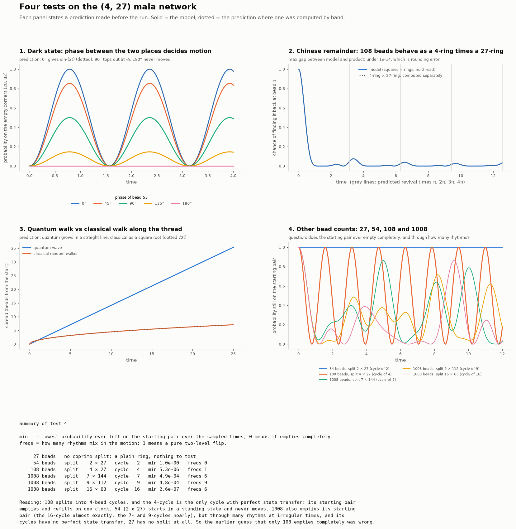
Four predictions were written down first, then run. Phase between two places decides whether anything moves at all. With square and ring hopping, the 108-bead network behaves exactly like a 4-bead ring and a 27-bead ring running together, because 4 and 27 share no factor. A quantum wave spreads in a straight line while a classical walker spreads as a square root. Among common mala counts, 108 is the only one whose split gives rings of beads where the particle can move from one corner to the opposite corner with certainty, a property called perfect state transfer that among rings only the four-bead one has. The guess that only 108 empties completely was wrong, and the record says so.
Technical
Numbers below are from a fresh run of the replication script, which CI checks against the published answer key on every change. Protocol and code are on the replication page; the original run is experiment-2-four-tests.py with its log quantum-tests-2-log.json.
Test 1, the dark state. Squares only, ψ(0) = (|0⟩ + e^(iφ)|54⟩)/√2. Prediction: P_empty(t) = cos²(φ/2)·sin²(2t) on beads 28 and 82. Maximum over 0 ≤ t ≤ 4:
| phase φ | 0° | 45° | 90° | 135° | 180° |
|---|---|---|---|---|---|
| max P_empty | 1.0000 | 0.8536 | 0.5000 | 0.1464 | < 10⁻³⁰ |
| cos²(φ/2) | 1 | 0.8536 | 0.5 | 0.1464 | 0 |
The first maximum at φ = 0 falls at t = π/4 ≈ 0.785. The state (|1⟩ − |55⟩)/√2 is an eigenvector of the 4-cycle Hamiltonian with eigenvalue 0, so it is stationary; the symmetric combination (|1⟩ + |55⟩)/√2 oscillates with P_empty = sin²(2t). A general phase φ mixes the two with weights cos²(φ/2) and sin²(φ/2), which is the prediction above. At 180° only the stationary part remains, and nothing moves.
Test 2, the factorisation. Squares and rings, strength 1 each, thread off. The network is then the Cartesian product C₄ □ C₂₇, because ℤ₁₀₈ ≅ ℤ₄ × ℤ₂₇ by the Chinese remainder theorem (4 and 27 are coprime). The explicit relabelling is k = (27a + 4b) mod 108, with a ∈ {0, …, 3} and b ∈ {0, …, 26}: a step of 27 moves a by one and leaves b alone, and a step of 4 moves b by one and leaves a alone. Under it, H = H₄ ⊗ I₂₇ + I₄ ⊗ H₂₇ entry by entry, with H₄ and H₂₇ the nearest-neighbour rings; the independent replication verified this exactly. So the return probability factorises, F(t) = F₄(t)·F₂₇(t), with F₄(t) = cos⁴t. Largest gap over 2,000 samples of [0, 4π]: 2.8 × 10⁻¹⁵, which is rounding error. At t = π, 2π, 3π, 4π the 4-ring factor returns to 1 but the 27-ring factor does not, so F stays small: 0.0485, 0.0248, 0.0167, 0.0334.
Test 3, quantum walk and classical walk. Thread only. Spread from bead 1, measured along the ring:
| time | 5 | 10 | 20 | fit |
|---|---|---|---|---|
| quantum σ | 7.071 | 14.142 | 28.284 | 1.4142 · t |
| classical σ | 3.162 | 4.472 | 6.325 | 1.4142 · √t |
These are the textbook values σ = √2·t for the continuous-time quantum walk and σ = √(2t) for the classical random walk at rate 1 per neighbour: the wave spreads ballistically, the walker diffusively. Konno (2005) gives the limit theorem for the continuous-time walk on the line, where position grows linearly in time; Kempe (2003) sets the quantum and classical scalings side by side, there for the discrete-time walk.
Test 4, other bead counts. For each count N and each coprime split N = p × q with 2 ≤ p ≤ q, one hopping rule of step q joins the beads into p-cycles. The particle starts on bead 1 and the bead ⌊p/2⌋·q places on, and we record the lowest probability left on that starting pair over 0 ≤ t ≤ 12, and how many distinct frequencies carry more than 1% of its oscillation.
| N | split | cycle | lowest P_start | frequencies > 1% |
|---|---|---|---|---|
| 27 | none | |||
| 54 | 2 × 27 | 2 | 1.000 (never moves) | 0 |
| 108 | 4 × 27 | 4 | 0 (to the time grid) | 1 |
| 1008 | 7 × 144 | 7 | 0.00049 | 6 |
| 1008 | 9 × 112 | 9 | 0.00048 | 9 (or 7, see §10) |
| 1008 | 16 × 63 | 16 | 0.0000003 | 6 |
Among the common mala counts (27, 54, 108, 1008), 108 is the only one whose coprime split produces a cycle with perfect state transfer: its four-bead squares (section 8). The split of 54 joins the beads in pairs, and a pair transfers perfectly too, but trivially, since a pair has nowhere else to go (the two-site case in Christandl and colleagues, 2004): from bead 1 alone the particle reaches bead 28 with certainty at t = π/4. (With the protocol’s start on both beads of the pair, it never moves, which is the row above.) The cycles of 7, 9 and 16 beads from 1008 have no perfect state transfer.
The earlier guess, that only 108 empties its starting pair completely, was wrong: 1008 empties its pair almost completely too, the 16-cycle to within 10⁻⁶, but through six or more frequencies at irregular times. That emptying is a weaker and different thing from perfect state transfer. The guess is kept here, marked wrong, rather than deleted.
8. The Square Qubit
The cleanest result
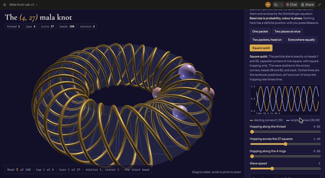
Start the particle on two opposite corners of one square. It drains completely into the other two corners and back, on a clock, forever. A classical random walker on the same square never does this: its chance of being on the starting corners never drops below a half. Start it on one corner alone and it arrives on the opposite corner with certainty. Physicists call this perfect state transfer, and among all ring-shaped networks only the four-bead one can do it.
Technical
Squares only, strength t_h. The square through bead 1 is the 4-cycle 1, 28, 55, 82. Write |S⟩ = (|1⟩ + |55⟩)/√2 and |E⟩ = (|28⟩ + |82⟩)/√2. Then H|S⟩ = −2t_h|E⟩ and H|E⟩ = −2t_h|S⟩, a two-level system with coupling 2t_h, while (|1⟩ − |55⟩)/√2 has eigenvalue 0 and never moves. Starting from (|1⟩ + e^(iφ)|55⟩)/√2, the weight on |S⟩ is cos²(φ/2), so
P_empty(t) = cos²(φ/2) · sin²(2t_h t)
a Rabi oscillation of period π/(2t_h). At φ = 0 it empties the starting corners completely; at φ = 180° the start is an eigenvector, the dark state of test 1. For the classical walker on one square, the chance on the starting corners is (1 + e^(−4t))/2.
Perfect state transfer. The 4-cycle is the Cayley graph of ℤ₄ and also the 2-dimensional cube (for perfect state transfer on cube-like graphs, see Cheung and Godsil, 2011). Start the particle on a single corner, at unit hopping, and the probability on the opposite corner is P(t) = sin⁴(t): it arrives with fidelity 1 at t = π/2, and again with period π. This is perfect state transfer (Christandl, Datta, Ekert and Landahl, 2004; Godsil, 2012, surveys the theory), and among the cycles Cₙ under the continuous-time walk, only n = 4 has it (Barr, Proctor, Allen and Kendon, 2014; also recorded by Dutta, 2022). Square hopping leaves the 27 squares disconnected, so 27 independent copies run in parallel. The site’s test recomputes P(π/2) on every change.
On a real quantum computer
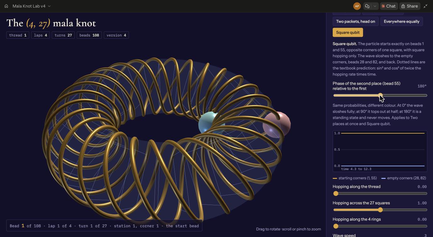
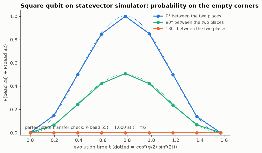
We ran the square on a real quantum computer, IBM’s ibm_kingston, on September 23, 2026. The particle placed on one corner arrived at the opposite corner 98 times in 100. Starting on two opposite corners in step, the empty corners filled to 99 percent at the predicted moment. Starting the same two corners out of step, nothing moved: the empty corners stayed at about 1 percent, which is the machine’s own error, the same 1 percent it shows when nothing has happened at all. The curves have the shape the formula predicts, with real-device noise on top. This is a demonstration, not a discovery: physicists have known this behaviour for more than twenty years. What it adds is that the mala’s square behaves on real hardware the way the page says it does.
- 0°, in step
- 90°
- 180°, out of step
- prediction
Perfect state transfer check, one corner to the opposite corner at t = π/2: P(bead 55) = 0.9815 (prediction 1).
The numbers
| t | 0° measured / predicted | 90° measured / predicted | 180° measured / predicted |
|---|---|---|---|
| 0.000 | 0.0090 / 0.0000 | 0.0105 / 0.0000 | 0.0085 / 0.0000 |
| 0.196 | 0.1415 / 0.1464 | 0.0748 / 0.0732 | 0.0088 / 0.0000 |
| 0.393 | 0.5222 / 0.5000 | 0.2465 / 0.2500 | 0.0122 / 0.0000 |
| 0.589 | 0.8327 / 0.8536 | 0.4535 / 0.4268 | 0.0180 / 0.0000 |
| 0.785 | 0.9890 / 1.0000 | 0.5240 / 0.5000 | 0.0103 / 0.0000 |
| 0.982 | 0.8353 / 0.8536 | 0.4370 / 0.4268 | 0.0173 / 0.0000 |
| 1.178 | 0.5092 / 0.5000 | 0.2595 / 0.2500 | 0.0155 / 0.0000 |
| 1.374 | 0.1427 / 0.1464 | 0.0880 / 0.0732 | 0.0115 / 0.0000 |
| 1.571 | 0.0075 / 0.0000 | 0.0097 / 0.0000 | 0.0110 / 0.0000 |
4000 shots per point, on ibm_kingston.
IBM ibm_kingston, September 23, 2026, 4000 shots per point, job daq3rdeekp0c73aq6aig. Dotted lines are the prediction cos²(φ/2)·sin²(2t). The evolution is two single-qubit rotations; the result is expected and known. It is here because a claim on this page was checked on a machine rather than in a simulation.
Technical
Two-qubit encoding of the 4-cycle (the 2-cube): |00⟩ = bead 1, |01⟩ = bead 28, |11⟩ = bead 55, |10⟩ = bead 82; H = −(X₀ + X₁); exp(−iHt) = RX(−2t) ⊗ RX(−2t). “Two places at once” is the Bell state (|00⟩ + e^(iφ)|11⟩)/√2, prepared by a Hadamard gate, CX and RZ(φ). Measured P(01) + P(10) against cos²(φ/2)·sin²(2t) for φ ∈ {0°, 90°, 180°}, t ∈ [0, π/2] in 9 steps, 4000 shots each; transfer check RX(−π) ⊗ RX(−π) on |00⟩.
Results on ibm_kingston: transfer 0.9815; 0° peak 0.9890 at π/4; 180° mean 0.0126 against a t = 0 floor of 0.0085 to 0.0105 (the three phases before any evolution, so state preparation and readout error); mean absolute deviation 0.012, max 0.027 (90°, t = 0.589). Shot noise at 4000 shots is about 0.008 near p = 0.5, so the largest residuals are device error (gate, phase, readout), not sampling. Transpiled with optimization level 3; job daq3rdeekp0c73aq6aig. Script, data, both plots and the run notes: square_qubit_ibm.py, square_qubit_results.json, run-notes.md.
9. Placement
Where the squares sit
The four beads of each little square are 27 apart along the thread, but on the knot they sit side by side, at the four corners of the tube. Wind a chain of quantum parts into this knot and each part gains a neighbour it never had in a straight line: the one across the tube. When the tube is thin, that is its nearest neighbour, and that is where the perfect flip would come from in a real device; it is the part of this page we could not find anywhere else. When the tube is fat, the same corner one step round the ring is nearer still, and the flip would be lost. Computed from the knot’s own geometry, the switch between the two is sharp, near a tube of 0.12 to 0.15 of the ring. On a thin tube, less than about a tenth of the ring, the squares are the closest thing to each bead and the flip survives: on its first pass it reaches 94 to 96 percent for a Rydberg-type coupling, and on the thinnest tubes it completes if you wait longer, because the square’s own diagonal slows it down. On a fat torus like the one the lab draws by default, the coupling runs along the ring instead and the squares disappear.
- 1/d⁶, Rydberg-type
- 1/d³, dipolar
- bead 29, next station
- bead 2, next along the thread
Best chance of bead 1 reaching bead 55, 0 ≤ t ≤ 40
Distance from bead 1 ÷ distance to its square partner, bead 28 (log scale)
The numbers
| tube ÷ ring | P(55), 1/d⁶ | P(55), 1/d³ | bead 29 ÷ bead 28 | bead 2 ÷ bead 28 |
|---|---|---|---|---|
| 0.02 | 1.000 | 0.982 | 8.373 | 8.351 |
| 0.03 | 1.000 | 0.895 | 5.637 | 5.643 |
| 0.04 | 1.000 | 0.802 | 4.269 | 4.304 |
| 0.05 | 0.999 | 0.770 | 3.448 | 3.510 |
| 0.06 | 0.996 | 0.714 | 2.901 | 2.989 |
| 0.07 | 0.977 | 0.685 | 2.510 | 2.624 |
| 0.08 | 0.961 | 0.636 | 2.216 | 2.356 |
| 0.09 | 0.956 | 0.566 | 1.988 | 2.151 |
| 0.10 | 0.940 | 0.542 | 1.806 | 1.991 |
| 0.11 | 0.896 | 0.522 | 1.657 | 1.864 |
| 0.12 | 0.784 | 0.403 | 1.532 | 1.760 |
| 0.13 | 0.565 | 0.240 | 1.427 | 1.674 |
| 0.14 | 0.292 | 0.111 | 1.337 | 1.602 |
| 0.15 | 0.123 | 0.099 | 1.259 | 1.542 |
| 0.16 | 0.047 | 0.062 | 1.190 | 1.490 |
| 0.17 | 0.040 | 0.073 | 1.130 | 1.446 |
| 0.18 | 0.027 | 0.057 | 1.076 | 1.408 |
| 0.19 | 0.020 | 0.066 | 1.028 | 1.374 |
| 0.20 | 0.010 | 0.060 | 0.985 | 1.345 |
| 0.21 | 0.006 | 0.045 | 0.946 | 1.319 |
| 0.22 | 0.003 | 0.039 | 0.910 | 1.296 |
| 0.23 | 0.001 | 0.035 | 0.878 | 1.275 |
| 0.24 | < 0.001 | 0.021 | 0.848 | 1.257 |
| 0.25 | < 0.001 | 0.029 | 0.821 | 1.241 |
| 0.26 | < 0.001 | 0.016 | 0.796 | 1.226 |
| 0.27 | < 0.001 | 0.015 | 0.772 | 1.212 |
| 0.28 | < 0.001 | 0.011 | 0.751 | 1.200 |
| 0.29 | < 0.001 | 0.009 | 0.730 | 1.189 |
| 0.30 | < 0.001 | 0.006 | 0.711 | 1.179 |
| 0.31 | < 0.001 | 0.005 | 0.694 | 1.169 |
| 0.32 | < 0.001 | 0.003 | 0.677 | 1.161 |
| 0.33 | < 0.001 | 0.002 | 0.662 | 1.153 |
| 0.34 | < 0.001 | 0.001 | 0.647 | 1.146 |
| 0.35 | < 0.001 | < 0.001 | 0.633 | 1.139 |
| 0.36 | < 0.001 | < 0.001 | 0.620 | 1.133 |
| 0.37 | < 0.001 | < 0.001 | 0.608 | 1.127 |
| 0.38 | < 0.001 | < 0.001 | 0.596 | 1.121 |
| 0.39 | < 0.001 | < 0.001 | 0.585 | 1.116 |
| 0.40 | < 0.001 | < 0.001 | 0.575 | 1.112 |
| 0.41 | < 0.001 | < 0.001 | 0.565 | 1.107 |
| 0.42 | < 0.001 | < 0.001 | 0.555 | 1.103 |
| 0.43 | < 0.001 | < 0.001 | 0.546 | 1.099 |
| 0.44 | < 0.001 | < 0.001 | 0.537 | 1.096 |
| 0.45 | < 0.001 | < 0.001 | 0.529 | 1.092 |
Above: the best chance of bead 1 reaching bead 55 as the tube gets thicker, with couplings set by real distance. Below: how close the next station and the next thread bead are to bead 1, compared with its square partner. When the bead 29 line drops below 1, the square is no longer the nearest structure.
Technical
Bead k and beads k ± 27 share a station (k mod 27) and sit on adjacent corners of the tube (27 ≡ −1 mod 4): the circulant chord of length 27 is realised as a spatially local coupling across the tube. The graph it makes, C₁₀₈(27) = 27 · C₄, is standard: 27 disconnected copies of the 4-cycle, whose perfect state transfer is section 8’s. (Bašić, 2011, characterises perfect state transfer on connected integral circulant graphs; this graph is disconnected, so it sits outside that theorem and needs only the 4-cycle result.) Models of helical molecules already let sites couple to their neighbours on the next turn (Guo and Sun, 2014, for electron transport). What we did not find, as far as we could find, is a torus-knot winding that makes the chord of 27 spatially local and reads it as the 27 four-cycles that carry perfect state transfer. Other nearest work: Biswas and Ghosh (2019), a continuous particle on a torus knot, with no sites; Gualdi, Kostak, Marzoli and Tombesi (2008), near-perfect transfer in a long-range, dipolar-like chain by removing the sender’s and receiver’s nearest neighbours.
Which bead is nearest depends on the tube. Mean distances between beads, measured on the lab’s own torus with ring radius 1:
| tube radius | k ± 27 (square) | k ± 28 | k ± 26 | k ± 54 (diagonal) | nearest is the square |
|---|---|---|---|---|---|
| 0.40 (lab default) | 0.566 | 0.232 | 0.830 | 0.800 | 0% of beads |
| 0.15 | 0.212 | 0.232 | 0.379 | 0.300 | 75% |
| 0.10 | 0.141 | 0.232 | 0.306 | 0.200 | 100% |
| 0.05 | 0.071 | 0.232 | 0.253 | 0.100 | 100% |
Bead k ± 28 is the same corner at the next station. It is the nearest bead of all at the lab’s default proportions, and the square’s corners are every bead’s nearest neighbours only when the tube radius is below 0.141 of the ring radius. Bead k ± 26 (the opposite corner at the next station) is always farther than k ± 27.
Our check, in one simple model. This is the only place on this page where geometry enters the equations; the lab’s hopping modes and Experiments 1 and 2 use the three hopping rules alone. The lab’s Couplings from distance mode (v5) runs the every-pair model below live, and its Wound chain preset shows the transfer appear as the tube thins. Let every pair of beads couple with strength (d₂₇/d)^α, normalised to the square’s edge, for distances below 2.5 bead spacings, with α = 3 (a dipolar fall-off) or α = 6 (Rydberg-type), and evolve for 0 ≤ t ≤ 40:
| tube radius | k ± 28 coupling, 1/d³ | square qubit, best P_empty, 1/d³ | one corner to bead 55, best, 1/d³ | one corner to bead 55, best, 1/d⁶ |
|---|---|---|---|---|
| 0.40 (lab default) | 5.27 | 0.011 | 0.000 | 0.000 |
| 0.25 | 1.81 | 0.069 | 0.022 | 0.000 |
| 0.15 | 0.50 | 0.329 | 0.107 | 0.124 |
| 0.10 | 0.17 | 0.799 | 0.554 | 0.940 |
| 0.08 | 0.09 | 0.926 | 0.635 | 0.961 |
| 0.05 | 0.02 | 0.994 | 0.770 | 0.999 |
| 0.02 | 0.00 | 1.000 | 0.982 | 1.000 |
At the default proportions the rings of k ± 28 dominate and neither effect appears. In a thin winding the square qubit comes back almost fully. The one-corner transfer is slowed by the coupling across the square’s diagonal (k ± 54), which is (√2/2)^α of the edge at every tube size: 0.354 under 1/d³, 0.125 under 1/d⁶. On a lone square that diagonal does not stop the transfer but delays it. The first pass, near t = π/2, reaches 0.738 under 1/d³ and cos²(π/16) = 0.962 under 1/d⁶; the first arrival above 0.999 comes at t ≈ 26.7 and t = 4π ≈ 12.6. On the knot, the weak couplings along the ring act during that wait, so the transfer completes only on the thinnest tubes. That diagonal leaves the square qubit alone: it shifts the two symmetric states (|1⟩ + |55⟩)/√2 and (|28⟩ + |82⟩)/√2 by the same amount. These are our computations in a model we chose, not a result from the literature. Script and output: wound-chain-check.py.
Every pair, no cutoff. The figure repeats the check with all couplings J = d^(−α), no cutoff, normalised to the bead 1 to bead 28 coupling: start on bead 1, record the best P(55) for 0 ≤ t ≤ 40. It agrees with the table to within 0.012; the only difference is the cutoff. The geometry behind it: each step along the thread is a quarter turn of the tube, so a square’s edge is a chord of √2·r ≈ 1.41 r; stations are 2π/27 ≈ 0.23 of the ring radius apart on average, more on the outside of the tube, where bead 1 sits, and less on the inside; bead k + 28 is the same corner at the next station. The switch falls between tube radii of 0.12 and 0.15; at the lab default of 0.4, P(55) < 10⁻³ under both laws. The r → 0 limit is not ideal square hopping, because the diagonal stays; it delays the transfer, as above. A first-pass run to t = 8 gives 0.962 and 0.879 at a tube of 0.02 and is kept as a file. Script and data: experiment-3-leak-geometry.py, leak-test-geometry.json, leak-test-geometry-first-pass.json.
Open. For two isotropic coupling laws, the threshold is computed above. Whether the transfer survives a physical winding with realistic couplings (anisotropic dipoles, exchange that falls off exponentially, disorder in the bead positions) is unanswered. It would make a good student project.
10. Replication
Independent replication
We handed the written recipe, with no answers, to a different AI system. It rebuilt the model from the description and got the same numbers.
Technical
The replication protocol defines the model and the four tests of Experiment 2, and asks for specific numbers; it contains no results and no predictions. It was given to ChatGPT, which implemented the model from the description, reproduced every requested quantity, and derived the factorisation of test 2 entry by entry. One count differed: for the 9-cycle of 1008 it found 7 frequencies above 1% where our run finds 9. The protocol allowed any reasonable weighting for that count, and no conclusion on this page depends on it.
One correction to our own record. The answer key’s classical spread at t = 20, 6.32454, was read off a 120-point time grid by linear interpolation; the exact value is √40 = 6.32456. The difference, 1.4 × 10⁻⁵, changes no conclusion, and the key is published unaltered.
You can run the same check yourself: the replication page has the protocol, the script and the answer key.
11. Scope
What this does and does not claim
It claims: that 108 = 2² × 3³ has exactly one split into coprime parts, 4 × 27; that 108 evenly spaced beads therefore sit on a single (4, 27) torus knot with one bead on each point of the 4 × 27 grid; that joining every n-th bead gives gcd(n, 108) polygons that survive any bending; that the same one-line rule appears in Chokwe sona, Tamil kolam and the Turk’s head knot; that the quantum mode is a standard one-particle system whose results were reproduced independently from a written description; and that the square-qubit behaviour is the known phenomenon of perfect state transfer on the 4-cycle, the only cycle that has it.
It does not claim: anything about consciousness, the brain, HCM or any theory on this site; that the quantum mode models a mala or a person; that any tradition chose 108 for its mathematics; that the thread’s shape has any physical effect; or that a number preserved in myth carries a hidden truth. The number came from the calendar. The mathematics came later, from elsewhere, and is ours to enjoy, not to overread.
12. How It Could Lose
What would show this is wrong
Find a second way to write 108 as two coprime factors, both greater than 1 (there is none, by arithmetic). Show a bending of the thread that breaks a shape (it cannot; the addresses are topological). Run the replication protocol and get numbers that differ beyond the stated tolerances. Show that the square-qubit trace departs from cos²(φ/2)·sin²(2t). Find prior work that places the chord-27 coupling on a wound chain as a spatially local coupling; we would cite it and drop the “not in the literature” line. Compute the bead distances on the (4, 27) knot yourself and find a fat-torus geometry (tube above 0.2 of the ring) in which the bead-1-to-bead-55 transfer exceeds 0.1 under 1/d³ or 1/d⁶ couplings; we found none. Any of these would discredit the page and we would say so here.
13. Credits and Files
Sources, credits and every file
Built by Dogma Guru with an AI counterpart (Claude, as Mantri) in September 2026; independently replicated by a second AI system.
Hardware run on IBM Quantum (ibm_kingston) under the Open plan, September 23, 2026.
Files
- quantum-experiment-report.png, quantum-experiment-log.json, experiment-1-two-places.py: Experiment 1.
- quantum-tests-2-report.png, quantum-tests-2-log.json, experiment-2-four-tests.py: Experiment 2.
- replication-protocol.md, replicate_mala_tests.py, answer-key.json: replication.
- square_qubit_ibm.py, square_qubit_results.json, square_qubit_results_ideal.json, square_qubit_plot.png, square_qubit_plot_ideal.png, run-notes.md, hardware-run-1.log: the square qubit on IBM hardware, and the simulator control.
- wound-chain-check.py: where the squares sit, and the distance check with a cutoff.
- experiment-3-leak-geometry.py, leak-test-geometry.json, leak-test-geometry-first-pass.json: the distance check with every pair, to t = 40 and to t = 8.
- minimal-model-M4-27.md: the (4, 27) minimal-model table.
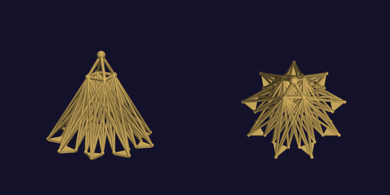
- 108-mala-knot.glb, .usdz, .stl, 108-meru.stl: 3D models.
- 108-geometry.png, 108-mala-knot.png, 108-meru-preview.png: figures.
Sources
- Ashley, C. W. (1944). The Ashley Book of Knots. Doubleday, Doran. Chapter 17, p. 233.
- Barr, K., Proctor, T., Allen, D., and Kendon, V. (2014). Periodicity and perfect state transfer in quantum walks on variants of cycles. Quantum Information and Computation 14(5&6), 417-438. arXiv:1204.5937.
- Bašić, M. (2011). Characterization of circulant graphs having perfect state transfer. arXiv:1104.1825; published as Characterization of quantum circulant networks having perfect state transfer, Quantum Information Processing 12, 345-364 (2013).
- Biswas, D., and Ghosh, S. (2019). Quantum mechanics of particle on a torus knot: curvature and torsion effects. arXiv:1908.06423; EPL 132, 10004.
- Cheung, W.-C., and Godsil, C. (2011). Perfect state transfer in cubelike graphs. Linear Algebra and its Applications 435(10), 2468-2474. arXiv:1010.4721.
- Christandl, M., Datta, N., Ekert, A., and Landahl, A. J. (2004). Perfect state transfer in quantum spin networks. Physical Review Letters 92, 187902. arXiv:quant-ph/0309131.
- Chuang, C., and Jin, B.-Y. (2014). Torus knots with polygonal faces. Proceedings of Bridges 2014, Seoul, 59-64. archive.bridgesmathart.org
- Di Prisa, A., and Şavk, O. (2026). Turk’s head knots and links: a survey. Expositiones Mathematicae 44, 125777. Preprint 2024, arXiv:2409.20106.
- Dresselhaus, E. J., Mahmoudi, S., Niu, L., Poincloux, S., Sanchez, V., and Dimitriyev, M. S. (2026). Textiles: from twisted yarn to topology and mechanics. arXiv:2604.09005.
- Dutta, S. (2022). Perfect state transfer using Markovian quantum walk. arXiv:2212.11699; Annals of Physics 488 (2026).
- Gerdes, P. (1988). On possible uses of traditional Angolan sand drawings in the mathematics classroom. Educational Studies in Mathematics 19(1), 3-22. doi:10.1007/BF00428382
- Gerdes, P. (1990). On mathematical elements in the Tchokwe “sona” tradition. For the Learning of Mathematics 10(1), 31-34.
- Godsil, C. (2012). State transfer on graphs. Discrete Mathematics 312(1), 129-147. arXiv:1102.4898.
- Grünbaum, B., and Shephard, G. C. (1980). Satins and twills: an introduction to the geometry of fabrics. Mathematics Magazine 53(3), 139-161.
- Grünbaum, B., and Shephard, G. C. (1988). Isonemal fabrics. American Mathematical Monthly 95(1), 5-30.
- Gualdi, G., Kostak, V., Marzoli, I., and Tombesi, P. (2008). Perfect state transfer in long-range interacting spin chains. Physical Review A 78, 022325. arXiv:0807.5018.
- Guo, A.-M., and Sun, Q.-F. (2014). Spin-dependent electron transport in protein-like single-helical molecules. Proceedings of the National Academy of Sciences 111, 11658.
- Hikami, K., and Kirillov, A. N. (2003). Torus knot and minimal model. Physics Letters B 575, 343-348. arXiv:hep-th/0308152.
- Ishimoto, Y. (2007). Solving infinite kolam in knot theory. Forma 22, 15-30. arXiv:0710.1976.
- Kempe, J. (2003). Quantum random walks: an introductory overview. Contemporary Physics 44, 307. arXiv:quant-ph/0303081.
- Konno, N. (2005). Limit theorem for continuous-time quantum walk on the line. Physical Review E 72, 026113. arXiv:quant-ph/0408140.
- Murasugi, K. (1991). On the braid index of alternating links. Transactions of the American Mathematical Society 326(1), 237-260.
- Siromoney, G., and Chandrasekaran, R. (1986). On understanding certain kolam designs. 2nd International Conference on Advances in Pattern Recognition and Digital Techniques, Indian Statistical Institute, Calcutta.
- Siromoney, G., Siromoney, R., and Krithivasan, K. (1974). Array grammars and kolam. Computer Graphics and Image Processing 3(1), 63-82.
- Yoshida, K. (2026). On isotopies and hyperbolicity of weaves. arXiv:2605.22129.